Explaining Time Complexity Of Algorithms Using The Big O Notation
Time complexity in algorithms determines its efficiency to solving problems. We can use the “Big O Notation” to determine the efficiency in approaching the problem. This is based off the runtime of an algorithm, that shows its complexity and performance. This describes how an algorithm scales with more inputs, as a way to classify algorithms and their response to changes in the input size. By knowing the efficiency of an algorithm, developers can build better applications.
We are going to look at how input scales the larger the data size. You will still get the same or similar result no matter what type of programming language or hardware is used. These are some of the more common types of the Big O.
Steps to determine the time complexity:
- Drop the less significant terms and identify the fastest growing term
- Drop the constants also called coefficients
Some Common "O" Notations:
Constant (“Order of 1”)
O(1) - Executes at the same amount of time no matter what size the data or what size the array is. It only requires 1 iteration to complete. The 1 can be any number, it is a constant.
T = N = c * 1 = O(1)
EX:
X = [A, B, C, D]
X[3] = D
There is no change in the time to search with the data set. When a defined array with values is already set, it just requires one iteration to find the data value. It will take a constant time, no matter what you are searching for in the data set.
Linear (“Order of N”)
O(N) - The time to complete is dependent or directly proportional to the number of items. For N the number of elements requires the same number of iterations to complete.
T = aN + B = N = O(N)
EX:
X = [A, B, D, E, F]
X.insert(2, C)
X = [A, B, C, D, E, F]
As you can see when we add the letter C in its proper position in the array, we had to move D, E and F 1 location to the right. That means X[n+1] so if the position of D is X[2] it will become X[2+1] or X{3] which is one position to the right. C will then assume the position X[2]. This required 3 additional operations for moving D, E and F.
Linear Search
Y = [apple, banana, mango, grapes, pineapple, durian]
If Target = “pineapple”, then the search will take a total of 5 tries, from apple to pineapple, before it gets the target from the array.
Quadratic (“Order of N Squared”)
O(N^2) - Time is measured as the square of N elements. The inputs are directly proportional to the exponential growth in time. It is quadratic in nature meaning the run time is proportional to the square root of the amount of data.
T = n*(n+1)/2 = n^2 + n/2 = O(N^2)
EX:
Bubble Sort
We want to sort an array in numerical order.
X = [21, 5, 3, 18, 30, 2, 8] -> X = [2, 3, 5, 8, 18, 21, 30]
First, X[0] compares itself to X[1], then X[2] until X[n], where n is the number of elements in the array. It will go down the entire row of elements until its position in the order is determined. Then X[1] will do the same thing and so on until the entire array is in numerical order. It must make multiple passes, compare adjacent indices and swap position with those that are out of order. This is the worst time complexity example in O notation.
Logarithmic (“Order of Log N”)
O(Log N) - In a logarithmic time scale doubling the size of the input data set has little effect on its growth. A single iteration just halves the input data so it is more efficient for handling large sets.
T = Log N^2 = O(Log N)
EX:
Binary Search
X = [10, 15, 35, 42, 60, 70, 82, 94]
If we want to set 60 as the target, the search will go to the middle half of the array and begin it’s search. Let’s say we go to position X[3] which is 42. If the target 60 is > x[3], eliminate the numbers below it in the array. If the target 60 < x[3], eliminate searches on the last part of the array. In this example anything below X[3] is eliminated leaving the search to start at X[4] which is the target we are looking for. It saves time when dealing with large arrays of data.
We can see that these are different approaches that can measure the efficiency of an algorithm. From observation we can see that over time as data gets larger and larger, the time to execute the code slows. Even if the processor on the computer gets faster, it won’t make the code execute any faster. Coding still requires efficiency and that matters especially when performance can improve productivity and reduce costs.

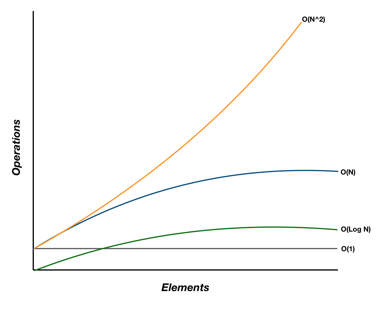
From the graph we can see that the complexity increases with more elements added since it increases the number of operations to run.
O(1) is constant, no matter how many elements are added the resulting operation will always be the same time.
O(N) is linear, it increases operations as the number of elements increases in direct proportion.
O(Log N) is half of linear time, it halves the number of operations required given the same elements as O(n).
O(N^2) shows the worst case scenario as operations increase steeply with the increase in number of elements.