LET: Low-Temperature Electron Transport | Chapter 4 - Results and Discussion (Part 1/2)
In the previous chapter, the experimental techniques explained how the experiment was carried out and why certain parts were carried out. This chapter will analyse the results from doing the experiment.

4 - Results and Discussion
The results of the experiment are to be presented and analysed. This section will delve into the Physics behind the results acquired.
4.1 Initial tests
The initial tests mentioned in the experimental techniques chapter have been carried out. These are to be analysed first.
4.1.1 - Choosing the optimum current
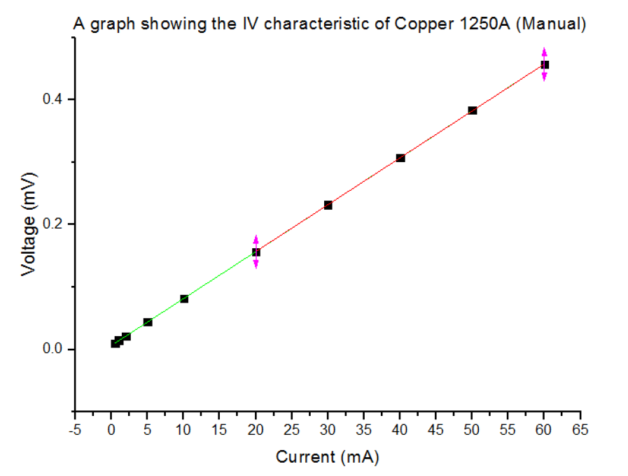
The first sample, Copper of thickness 1250Å, was placed on the probe stick. The current was then manually altered and the corresponding voltages were recorded. Figure 10 shows that from 20mA to 60mA, I∝V, therefore, any current in that range is suitable to use for the experiment. 30mA was chosen. Having chosen this current, a reistance-temperature measurement was recorded using the software.
4.1.2 - Using the Van der Pauw equation
As a test run, the resistivity of Copper, of thickness 1250Å, was calculated, at room temperature, using the Van der Paouw Equation. The correction factor was assumed to be 1 due to there being only 1 resistance value. Using equation X, the resistivity value calculated was ρ=0.425±0.0006μΩcm. The accepted value of the resistivity of copper at that particular thickness, room temperature, is ρ=1.68μΩcm [1]. The experimental value appeared to be an order of magnitude less than the book value, presumably due to the assumption that the correction factor was equal to 1. As will be shown; the correction factor plays a big part in ‘correcting’ the resistivity. Another uncertainty which causes this value to be innacurate, is that the contact points of the pins and sample are in the middle, as opposed to around their sides. This is a limitation as resistivity changes with the size of a material; in this experiment’s case, it is best to have the contact points in a fixed position, as the sample size varies – i.e. not all the samples are the exact same size.
4.2 - Metal Samples
Five samples of Copper, of different thicknesses, were scanned for their IV characteristic and variation of resistance with temperature. A suitable current of 30mA was consistently used throughout each metal sample of each thickness.
4.2.1 - Copper (1250Å)
Since an IV characteristic was already obtained for Copper of this thickness, in section 4.1.1, this step was not repeated. As previously mentioned in section 3.5, two resistances were obtained, with their temperatures, from the rotation of pin configuration method. These resistances were:
This gave a ratio R2/R1=9.567. By referring to the correction factor graph, this ratio resulted in f=0.7. Now, using the Van der Pauw equation, a resistivity of ρ=1.57±0.06μΩcm was calculated. As mentioned before, the book value of Copper, of thickness 1250Å, is ρ=1.68μΩcm, at room temperature [1]. This proves that the correction factor is vital for eliminating any inconsistencies in the sample and allowing a more accurate resistivity to be calculated. Though the calculated resistivity is a lot closer to the book value; the book value does not lie in the upper-bound of the calculated uncertainty. Since the value is very close, this could be due to neglecting or simplifying the uncertainty, as shown in the appendix. Alternatively, this could be due to the pins on the probe-stick being in the middle of the sample rather than around its edges, as mentioned previously. After calculating the resistivity using the Van der Pauw equation, the probe stick with the sample is dipped and a resistance vs temperature graph is computed by the program.
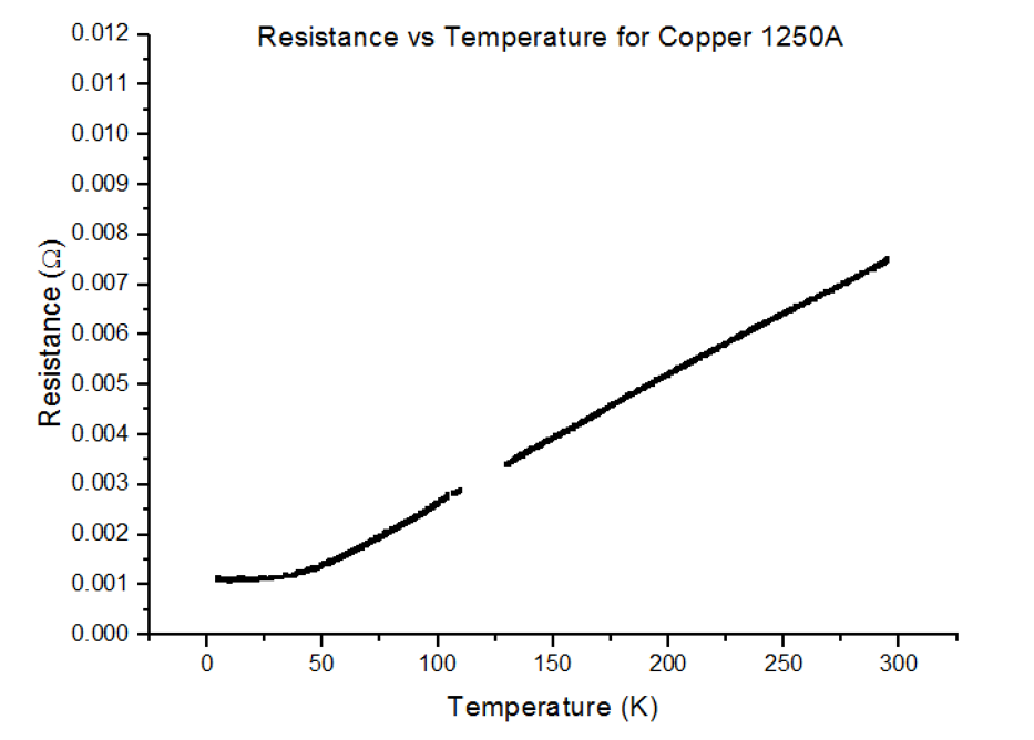
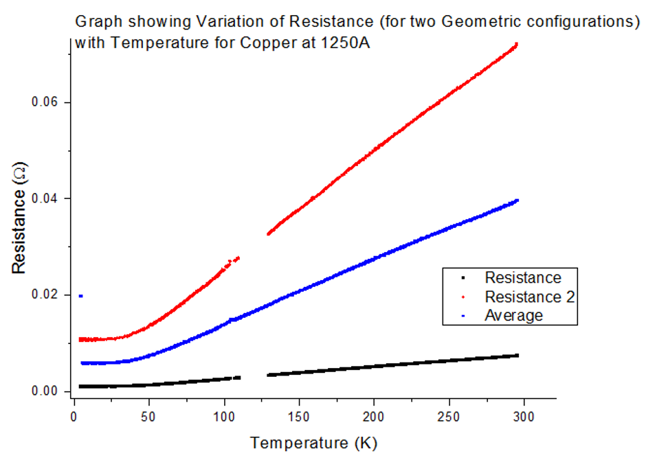
Since the data in figure 11 is data for one of the two pin configurations, the second resistance is used to extrapolate and an average of the two is then obtained as shown in figure 12, below.
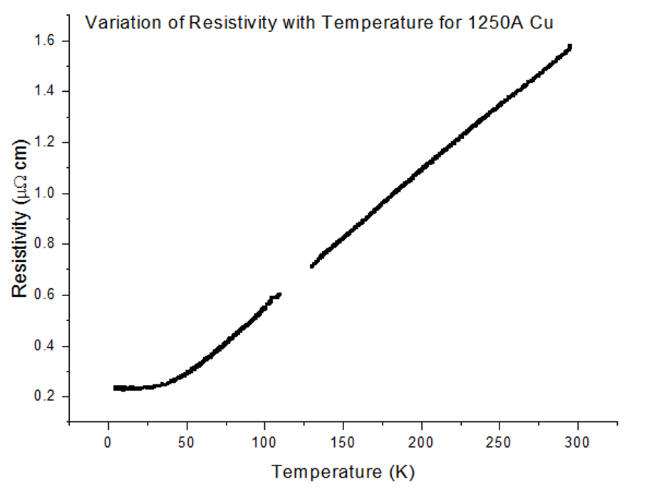
The average resistance values in figure 12 were then converted into resistivity values using the Van der Pauw equation and plotted as shown in figure 13.
This method was then repeated to obtain resistivity vs temperature graphs for several Copper samples of varying thicknesses, as shown below.
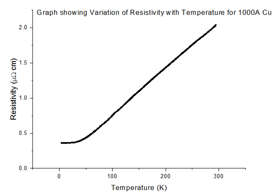
4.2.2 - Copper (1000Å)
The IV characteristic for Copper of 1000Å thickness was computed using a current of 30mA and an Ohmic relation was established. The two resistances acquired from the rotation of pin configuration are as follows:
These values gave a ratio R1/R2=1.025. This meant that the correction factor, f=1. The calculated resistivity from the Van der Pauw equation, using these values, was ρ=1.634±0.07μΩcm, at room temperature. The resistivity vs temperature graph was computed, as shown in figure 14.
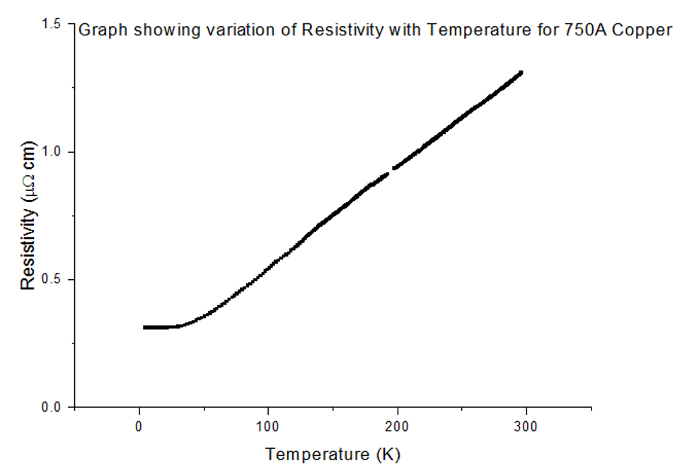
4.2.3 - Copper (750Å)
The two resistances acquired from the rotation of pin configuration are as follows:
These values gave a ratio R1/R2=1.3. This gave f=0.05. The calculated resistivity from the Van der Pauw equation, using these values, was ρ=1.70±0.07μΩcm, at room temperature. Having done these calculations and followed the correct steps mentioned; the resistivity vs temperature graph was computed, shown in figure 15.
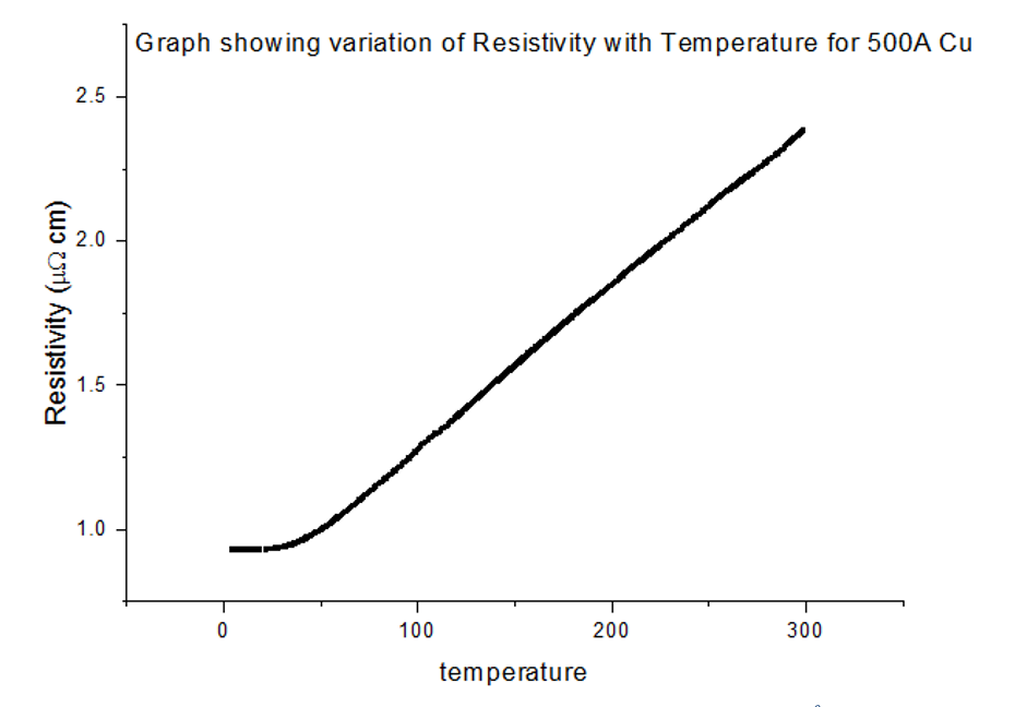
- 4.2.4 Copper (500Å)
The two resistances acquired from the rotation of pin configuration are as follows:
These values gave a ratio, R1/R2=1.27. This gave f=0.95. The calculated resistivity from the Van der Pauw equation, using these values, was ρ=1.714±0.07μΩcm, at room temperature. Having done these calculations and followed the steps mentioned; the resistivity vs temperature graph was computed, shown in figure 16.
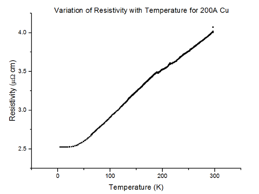
4.2.5 - Copper (200Å)
The two resistances acquired from the rotation of pin configuration are as follows:
These values gave a ratio, R1/R2=1.04. This gave f=1. The calculated resistivity from the Van der Pauw equation, using these values, was ρ=1.721±0.07μΩcm, at room temperature. Having done these calculations and followed the steps mentioned; the resistivity vs temperature graph was computed, shown in figure 17.
4.2.6 - Summary of Metals
All ρ-T graphs for Copper, of all thicknesses, followed the same trend as the Bloch Gruneisen function. As the temperature fell from 300K, the resistivity dropped linearly, where ρ∝T; then, at a certain temperature, the trend became similar to ρ∝T5. A few more Kelvin colder and there was no more temperature dependence, ρ∝T0, on the resistivity, as temperature dropped down to 4.2K
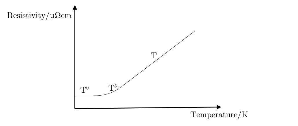
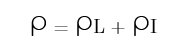
At such low temperatures, the resistivity no longer dropped further due to the electron-phonon scattering contribution, ρL, of the resistivity. The total resistivity is equal to the sum of the electron-phonon contribution to resistivity, ρL, and the impurity contribution to resistivity, ρI [2].
As the temperature tends to 0K, the electron-phonon scattering contribution, ρL, of the total resistivity also tends to 0
- ρL is the property that results in ρ∝T, where at a certain temperature, the trend becomes ρ∝T5. As previously mentioned, at low enough temperatures the relation becomes ρ∝T0.
- ρI, or the electron scattering due to impurities, is responsible for the flat line part of all of the Copper ρ-T graphs, where ρ∝T0.
Further analysis can also be done. By looking at the variation of the resistivity of the sample with the sample’s thickness, a trend can be observed. Two resistivity vs thickness graphs were plotted; one at room temperature and one at 4.2K. These graphs are shown below in figures 19 and 20.
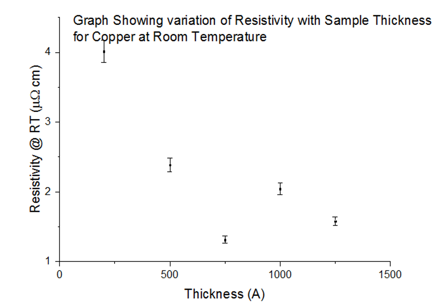

As can be seen, the resistivity of a given sample drops as its thickness decreases [3]. This is due to phonons having less room to propagate due to the very thin films that are being analysed in this experiment. Less room for phonon propagation reduces the electron-phonon scattering component of the total resistivity, thus, decreasing the resistivity for decreasing sample thickness. Said trend can be further analysed using the Fuchs Sondheimer relation, which will be discussed in section 4.2.8.
4.2.7 - Using the Bloch Gruneisen function
To further analyse the data acquired, a Bloch Gruneisen function can be fitted to calculate parameters such as the Debye temperature at a given thickness. The Debye temperature is the temperature of the crystal’s highest mode of vibration. The function is as follows:
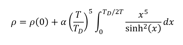
The integral in this function is the sum of all phonon models and it makes two assumptions [4]:
- Using 0 as the lower bound assumes that the material is large enough such that the lower limit from the maximum photon wavelength is equal to 0.
- Using an integral assumes a continuum of available modes such that variation between modes is sufficiently smooth.
Due to the complexity of this function, python was used to fit it to the data acquired for all thicknesses of Copper. The graphs produced from the code are shown with the code making up these graphs in the appendix. The Debye temperatures were then extracted and plotted on a Debye temperature vs thickness graph:
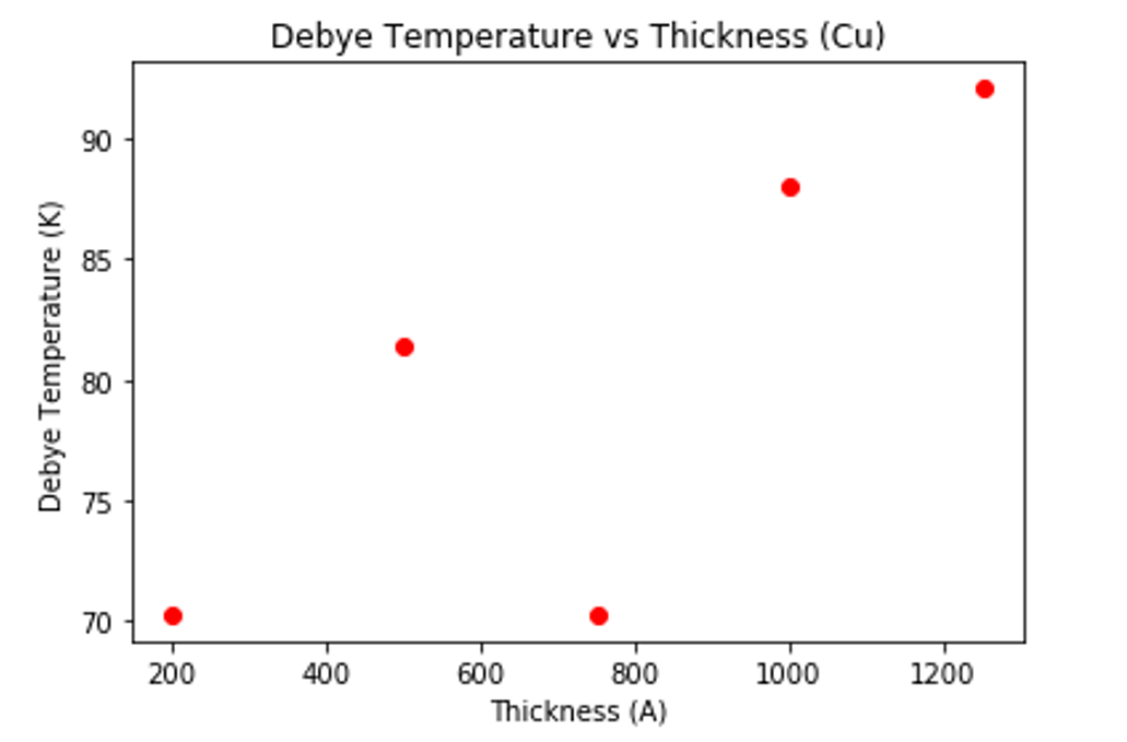
As the film thickness increases, the Debye temperature also increases. This is due to phonon softening, which is due to missing bonds at the film interface, leading to different vibrational amplitudes [5]. An anomaly was observed at Copper of thickness 750Å; it was determined to be due to the accidental use of a misplaced 200Å thickness sample amongst the 750Å samples.
4.2.8 - Using the Fuchs Sondheimer function
As can be seen from the resistivity vs thickness data in figures 19 and 20, there is a clear correlation. A Fuchs Sondheimer function is fit to the resistivity vs thickness data for even further analysis. The full complexity Fuchs Sondheimer function was coded, as shown in the appendix, but the program did not work. The problem was that there were 5 resistivity data points due to the 5 thicknesses of Copper in this experiment, one of which was an anomaly; therefore, the program was essentially asked to draw a correlation from 4 data points using such a complex function. A big simplification of the Fuchs Sondheimer model, shown below, was then used to compromise.
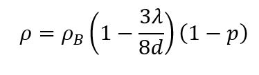
The reflectivity ratio, p, is a measure of how smooth the surface is and can be any value between 0 and 1. This parameter, p, is assumed to be 0, meaning the surface is completely smooth, for simplification. The bulk resistivity is the resistivity that is tended to as film thickness gets thicker and thicker. The new equation now becomes as follows:
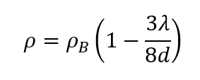
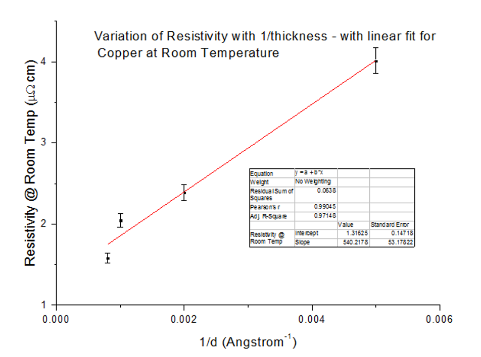
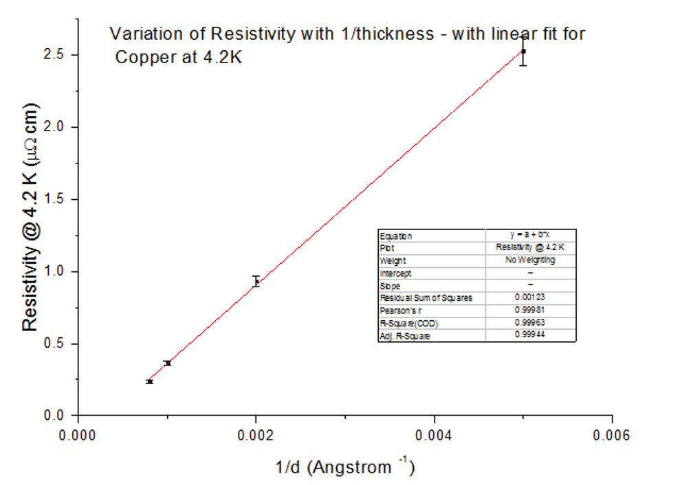
This equation is now in the form y=mx+c, meaning a graph of resistivity vs 1/thickness can be plotted. By fitting a straight line to this new graph and calculating the gradient, the bulk resistivity, ρB, and the mean free path, λ, can then be determined. The plots of the graphs are shown below at both room temperature and 4.2K, in figures 22 and 23, where the anomaly at 750Å has been removed.
Since the aforementioned simplification of the Fuchs Sondheimer equation is in the form y=mx+c; the gradient, m, and y-intercept, c, equate to:
The error of the y-intercept can be read directly off the fit on the graph, whereas the error of the mean free path, λ, is calculated by using the following equation:
Using these equations, the bulk resistivity and mean free path, from both graphs, can be calculated.
4.2.8.1 - Evaluation of Room Temperature graph
As quoted before, the book value of ρB for Copper ρ=1.68μΩcm, is very comparable to the value determined from the use of a simplified Fuchs Sondheimer model (for room temperature values). Although the book value did not lie in the bounds of the uncertainty, the value is still acceptable and accurate to some degree. The book value for the mean free path, λ=3x10⁻⁶cm [6], compared to the calculated experimental value, is within an order of magnitude.
4.2.8.2 - Evaluation of 4.2K graph
The calculated values for the low temperature 4.2K graph were much further from the book values. Firstly, the calculated bulk resistivity of Copper at this temperature was negative, which is not possible. Secondly, as temperatures become so low, the mean free path of Copper is considerably higher due to reduced electron-phonon interaction rates of around 0.3cm; the calculated value is multiple orders of magnitude lower than this. Such correlations at 4.2K can be due to the mean free path being much higher than the thickness of the sample; as a result, the Fuchs Sondheimer model breaks down due to surface scattering taking over. This allows us to draw two conclusions:
- The model is not perfect; it has been considerably simplified to suit the thin films data in this experiment, despite this simplification working well at room temperature.
- The effect of surface scattering becoming dominant cannot be neglected for the room temperature data as the mean free path is still considerably larger than the sample thickness, hence, an alternative model is required.
If you have any questions, leave them below and until next time, take care.
~ Mystifact
References:
[1]: Rosemburg, H. 1975. The Solid State, 5th ed. pp 241. England. Oxford University Press
[2]: Bass, J. 2006. Deviations from Matthiessen’s rule. [05/04/2018]. Available from: https://www.tandfonline.com/doi/abs/10.1080/00018737200101308
[3]: Lacy, F. 2011. Developing a theoretical relationship between electrical resistivity, temperature and film thickness for conductors. [10/04/2018]. Available from: https://www.ncbi.nlm.nih.gov/pmc/articles/PMC3284497/
[4]: Boekelheide, Z, et al. 2009. Resonant impurity scattering and electron-phonon scattering in the electrical resistivity of Cr thin films. [10/04/2018]. Available from: https://sites.lafayette.edu/boekelhz/files/2014/03/PhysRevB_80_134426.pdfhttps://sites.lafayette.edu/boekelhz/files/2014/03/PhysRevB_80_134426.pdf
[5]: Z, Cheng, et al. 2010. Phonon Softening and Weak Temperature-dependent Lorenz Number for Bio-supported Ultra-thin Ir Film. [08/10/2018]. Available from: https://arxiv.org/ftp/arxiv/papers/1410/1410.1912.pdf
[6]: Kittel, C. 2004. Introduction to Solid State Physics, 8th ed. pp276. USA. John Wiley & Sons
Please note; no copyright infringement is intended. All images used have been labelled for re-use on Google Images. If any artist or designer has any issues with any of the content used in this article, please don’t hesitate to contact me to correct the issue.
Previous LET chapters:
Chapter 2 - Introduction
Chapter 3 - Experimental Techniques
Follow me on: Facebook, Twitter and Instagram, and be sure to subscribe to my website!