NETWORK SYNTHESIS FOR SIGNAL FILTERING
DEFINITION OF NETWORK SYNTHESIS.
I allow myself to define the network synthesis as does Alexander Sadiku's book, which states that network synthesis is the process to obtain an appropriate network in order to represent a given transfer function. Network synthesis is easier to apply in the domain than in the time domain.
In the network analysis, we find the transfer function of a given network. In network synthesis we invert the process, that is; it is required that we find a convenient network that represents a given transfer function. Because the network synthesis consists of determining a network type that represents a given transfer function, we can affirm that there are many different answers or (possibly none) because there are many circuits that are used to represent the same transfer function, for the In the network analysis, there is only one response.
In the design of analog filters, both network analysis and the method of network synthesis are combined, network synthesis being the heart of the design of modern filters by the method of insertion losses.
The network synthesis is an entire course by itself and requires some experience and skill to find the most appropriate network to design requirements, but this article will only cover what is needed to design our filters. The network synthesis can be active or passive, depending on the nature of its elements.
The two examples are from Alexander Sadiku's book but the graphics were made with multisim and pain. This is basic to what I will show in future publications about my research in the math degree applied to the area of communications on the "advanced method of signal filtering by network synthesis using approximate polynomials". The polynomials with which both design, simulation and implementation works for both passive and active filters were: Butterworth, Chebishev Type I, Chebishev Type II, Legendre, Elipticos or Cauer, Laguerre, Hermite type I, Hermite Type II. I am currently working with the hyperbolic tangent function which is a pure lomito in the approach research for signal filtering.
Example 1: Given the following transfer function H (s), synthesize this function, using the passive circuit of figure 4.1: a) select for R = 5 Ω; find L and C b) select for the case of normalization R = 1 Ω; find L and C
H (s) = 10 / (s ^ 2 + 32s + 10) (Eq. 1.)
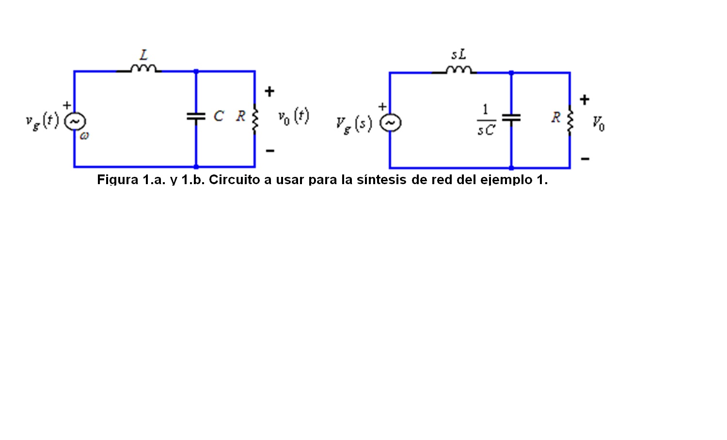
Solution: The equivalent in the domain of s for the circuit of figure 1.a, is shown in figure 1.b. We know by network arrangement that the parallel combination of R and C gives:
R║1 / sC; Zeq1 = R / (1 + sRC)
Using the voltage division principle, we obtain the following transfer function:
(V0(s)) / (Vi (s)) = (1/LC) / (s ^ 2 + s/RC + 1/LC) (Eq.2)
When comparing with the transfer function H (s) given in (Ec.1), with that obtained in the equation (Eq.2), it turns out that:
1 / LC = 10; 1 / RC = 3
a) Selecting R = 5, then we have:
C = 1 / 3R = 66.67 mF L = 1 / 10C = 1.5 H
b) Selecting R = 1 Ω, then that:
C = 1 / 3R = 0.333 F L = 1 / 10C = 0.3 H
Example 2: Given the following transfer function H (s), synthesize this function, using the active circuit of Figure 2.
H (s) = (10^ 6) / (s ^ 2 + 100s + 10 ^ 6) (Eq. 3)
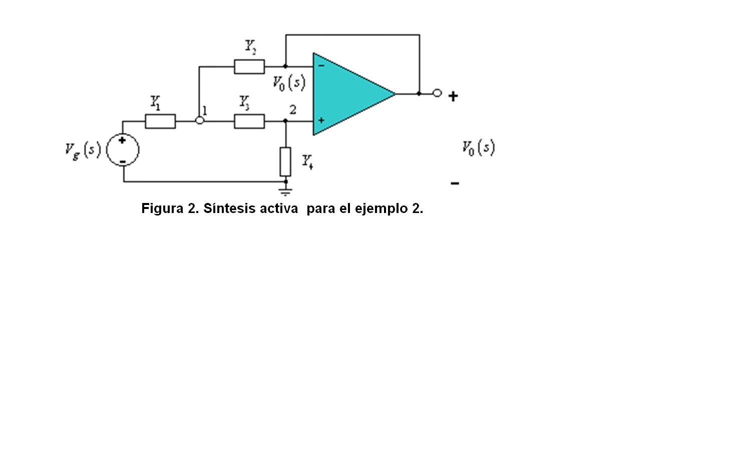
Applying nodal analysis in nodes 1 and 2 and using the virtual short circuit theory OPAMP, we obtain the following transfer function:
H (s) = (Y1Y3) / (Y1Y3 + Y4 (Y1 + Y2 + Y3)) (Eq.4)
To synthesize the transfer function H (s), given in equation 3, we compare it with the one obtained in equation 4. For this we must take into account two aspects: 1). Y1Y3 must not contain s, because the numerator of H (s) is constant. 2). The transfer function is second order, which implies that we must have two capacitors. Because of these two points, we must do Y1Y3 resistive and we do Y2Y4 capacitive. That is:
Y1 = 1 / R1 Y2 = sC1 Y3 = 1 / R2 Y4 = sC2 (Eq.5)
Substituting equation 5 in equation 4, developing and grouping the terms, we have then:
H(s)=(1 ⁄(R1R2C1C2))/(s^2+(s(R1+R2)) ⁄ (R1R2C1))+1 ⁄ (R1R2C1C2))) (Eq.6)
Comparing (6), with the given equation (3), we note that:
(1 ⁄(R1R2C1C2))=10^6 ((R1+R2) ⁄(R1R2C1))=100
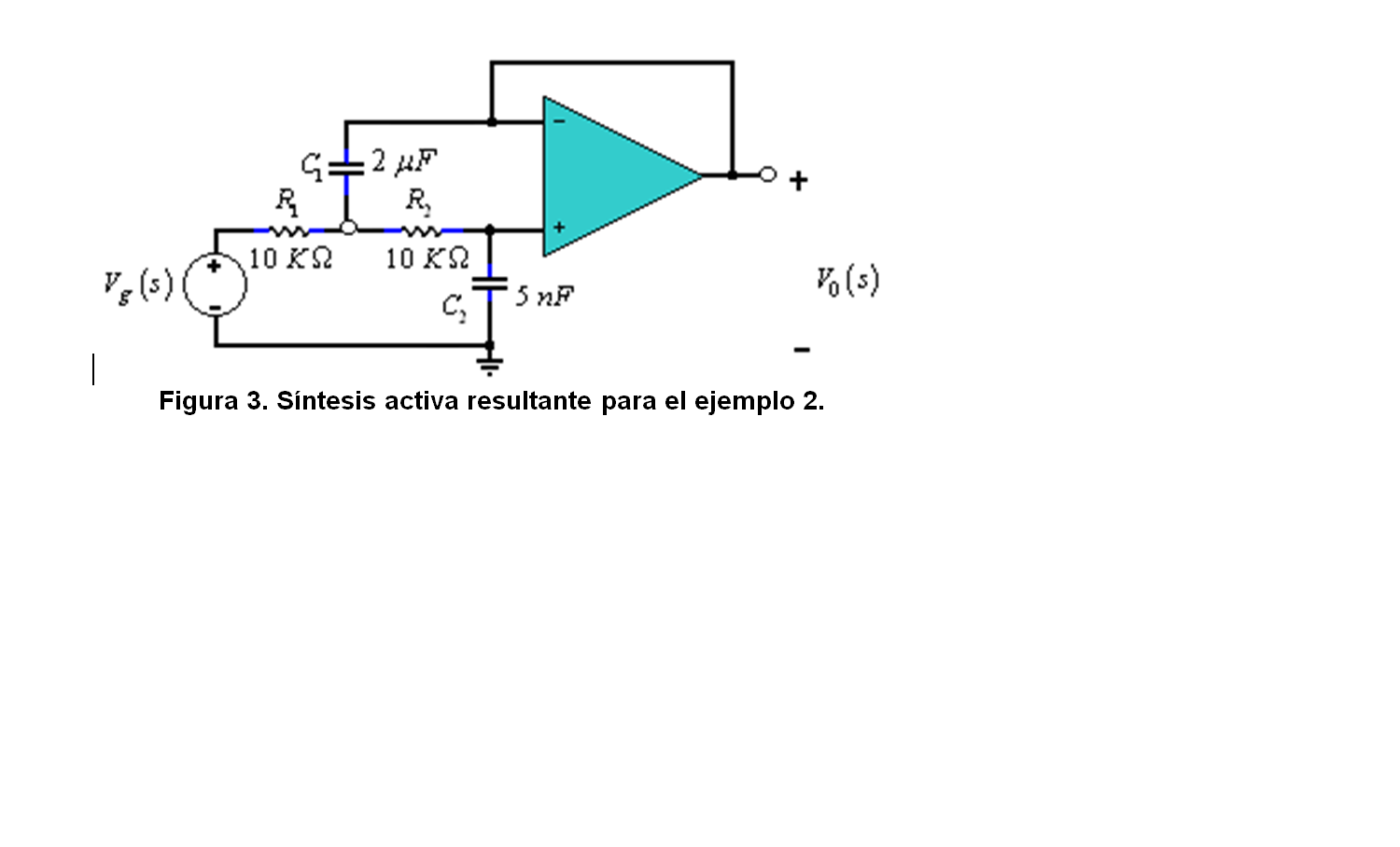
If we select R1 = R2 = 10 kΩ, then it results:
C1=((R1+R2)) ⁄((100R1R2)) = 2μF C2=(10^(-6)) ⁄(100R1R2C1))= 5 nF
The two examples are from Alexander Sadiku's book but the graphics were made with multisim and pain. This is basic to what I will show in future publications about my research in the math degree applied to the area of communications on the "advanced method of signal filtering by network synthesis using approximate polynomials". The polynomials with which both design, simulation and implementation works for both passive and active filters were: Butterworth, Chebishev Type I, Chebishev Type II, Legendre, Elipticos or Cauer, Laguerre, Hermite type I, Hermite Type II. I am currently working with the hyperbolic tangent function which is a pure lomito in the approach research for signal filtering.