Programming and Implementing the Red Pitaya Electronics Board For Signal Acquisition
Implement a feedback control system by using the Red Pitaya board to minimise the effect of fluctuations (noise) due to environmental conditions.
Self-Produced
Overview
The purpose of this experiment was to implement a feedback control system by using the Red Pitaya board (SoC = system on a chip; DAQ = data acquisition system). Feedback is omnipresent in quantum optics experiments, the boards purpose is to minimise the effect of fluctuations (noise) due to environmental conditions.

Introduction
The Red Pitaya [1] is an affordable field-programmable gate array (FPGA) board with fast analog inputs and outputs. This makes it useful for quantum optics experiments, in particular as a digital feedback controller for analog systems. Based on the open source software provided by the manufacturer of the board, I studied the software package PyRPL [2][3] (Python RedPitaya Lock-box) which implements many devices that are needed for optics experiments with the Red Pitaya.
The Red Pitaya and PyRPL
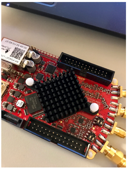
Figure 1: - The Red Pitaya
Self-Produced
The Red Pitaya board (recently renamed "STEMlab 125-14") was first released in 2013 as a kick-starter project and has since gained great popularity in the scientific and electronics communities. The board combines a Xilinx Zynq-7010 System-on-chip (SoC) [4] with two channel analog-to-digital (ADC) and digital-to-analog (DAC) converters with 14 bit resolution and 125 MHz sampling rate. The term SoC generally indicates that various systems are implemented on the same chip. In the case of the Zynq-7010, an FPGA allowing programmable logic (PL) is combined with a dual-core processing system (PS), composed of an ARM Cortex-A9 processor with standard peripherals such as memory and input-output interfaces, and a high-bandwidth connection to the FPGA.
PyRPL [5] is an open-source software package providing many instruments on cheap FPGA hardware boards, such as:
- oscilloscopes;
- network analyzers;
- lock-in amplifiers;
- multiple automatic feedback controllers;
- digital filters of very high order (24).
PyRPL currently runs exclusively on the Red Pitaya. PyRPL comes with a graphical user interface (GUI), but it also has a convenient Python application programming interface (API) on which the GUI is based. The user-interface and all high level functionality are written in Python, but an essential part of the software is hidden in a custom FPGA design written in the hardware description language Verilog.
GUI and API
Self-Produced
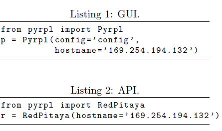
Once you have determined the IP address of your Red Pitaya, to start PyRPL's GUI, simply create a PyRPL object like in List 1. If you are using the "file config" for the first time, a screen will popup asking you to choose among the different Red Pitayas connected to your local network. After that, the main PyRPL widget will appear. The main PyRPL widget is initially empty, however, you can use the modules menu to populate it with module widgets. The module widgets can be closed or reopened at any time, docked/undocked from the main module window by drag-and-drop on their sidebar, and their position on screen will be saved in the configuration file for the next startup. Similarly, you will be able to connect to the API as done in List 2.
RedPitaya modules
The Red Pitaya contains different modules which are distinguished between hardware and software. The hardware modules represent the different sections of the FPGA and they are:
- r.hk -> housekeeping = LEDs and digital inputs/outputs;
- r.ams -> analog mixed signals = auxiliary ADCs and DACs;
- r.scope -> oscilloscope interface;
- r.asg -> arbitrary signal generator, two channels;
- r.pid -> three PID modules;
- r.iq -> three I+Q quadrature demodulation/modulation modules;
- r.iir -> infinite impulse response filter module that can realize complex transfer functions.
On the other hand, software modules are directly accessible at the root pyrpl object (no need to go through the redpitaya object). It is also possible to implement complex functionality in the Red Pitaya: in particular the Network Analyzer (NA), the Lorentzian band-pass filter and the frequency comparative module can be seen as three applications of the IQ module. I will present the modules that I used in this article.
PID
Proportional-integral-derivative controller is a control loop feedback mechanism. A PID controller continuously conditions the information contained in an error signal e(t) that comes from a physical system, subjected to unwanted perturbations. Thus it calculates e(t) as the difference between the input signal sin and a desired set-point s0 (e(t) = s_in - s_0), and applies a correction based on proportional, integral, and derivative terms (denoted P, I, and D respectively) which give their name to the controller. In practice, it automatically applies accurate and responsive correction to a control function. The overall control function of the output signal s_out can be expressed mathematically as shown in the equation below.
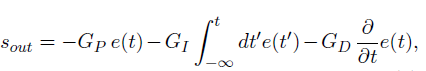
Where G_P , G_I and G_D all non-negative denote the coefficients for the proportional, integral, and derivative terms, respectively.
IIR - Infinite Impulse Response
The IIR module can implement filters with the following constrains:
- strictly proper transfer function;
- poles (zeros) either real or complex conjugate pairs;
- no three or more identical real poles (zeros);
- no two or more identical pairs of complex conjugate poles (zeros);
- pole and zero frequencies should be larger than nyquist-frequency/1000 (but you can optimise the nyquist frequency of your filter by tuning the loops parameter, whose definition will be given later on);
- the DC-gain of the filter must be 1.0;
- total filter order less than 16.
Beside that, a remaining bug limits the dynamic range to about 30 dB before internal saturation interferes with filter performance.
The operation of the module is regulated by the function in the Laplace domain.
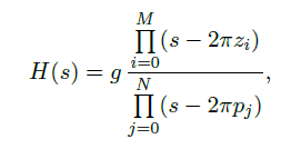
where g is a constant scaling factor, p_j are the complex poles and z_i the zeros of the transfer function: the last two are the parameters to plug into the program.
Experimental Results
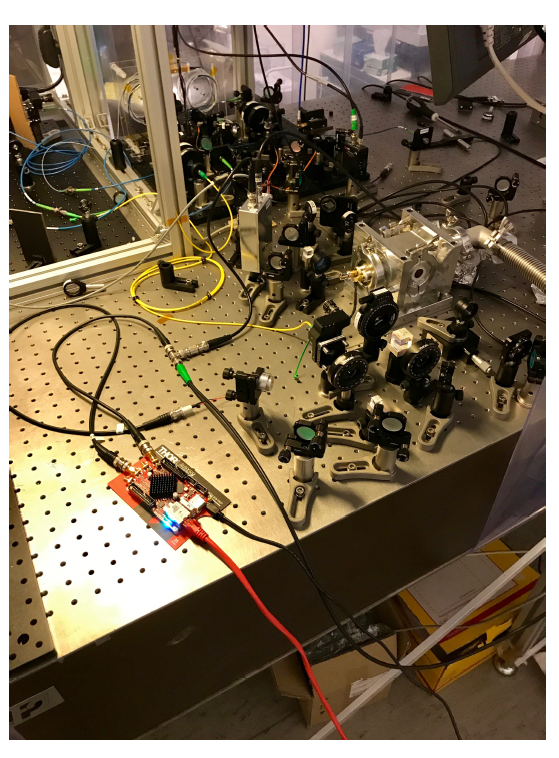
Photograph of my Experimental setup, with the optical components and the Red Pitaya.
Analog Low-pass Filter
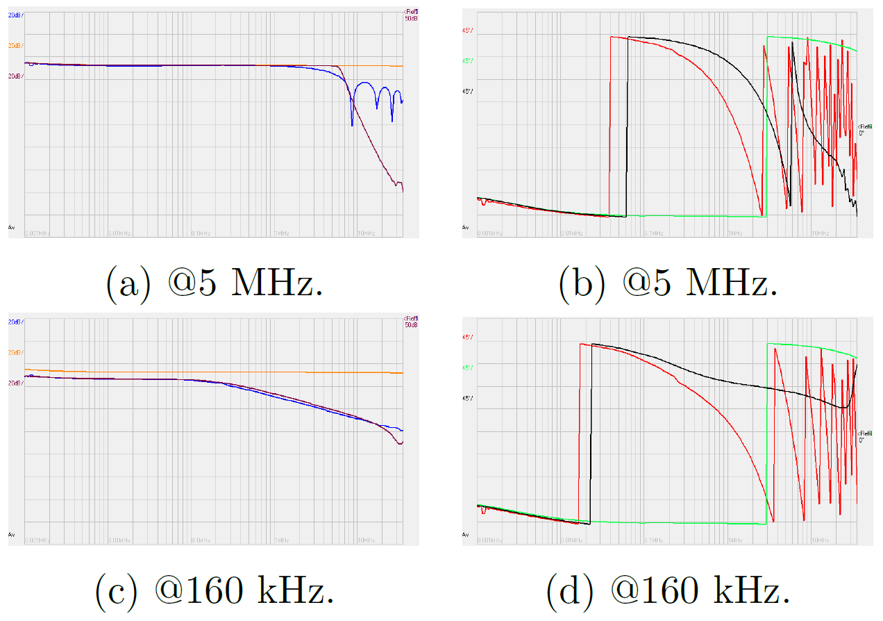
Figure 2: Network Analyzer response. Orange and green lines refer to the amplitude and phase when the output and the input of the NA are connected together for calibration, violet and black with a low-pass filter (whose cutoff frequency is indicated), blue and red to the Red Pitaya.
The transfer function of a low pass filter is:
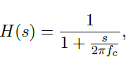
where fc is the cutoff frequency.
In Fig. 2 amplitude and phase of the signal of the Network Analyzer connected with itself, a low-pass filter, and the Red Pitaya are shown. In order to avoid "flooding", the attenuation level has been set to 3.1 dB and with a measurement time sufficiently long of about 10 s in order to correctly measure at low frequencies. So I tried to digitally replicate through the Red Pitaya the analog filter I had through the IIR module, via GUI. Since at frequencies ~ 10 MHz it started to oscillate, I chose a first order low-pass filter whose I estimated the cutoff frequency to be about 160 MHz.
Series of Low-pass Filters
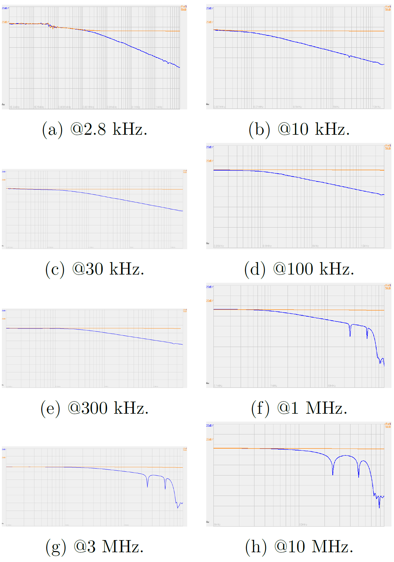
Figure 3: Series of low-pass filters. Below each chart the cutoff frequency of that filter is indicated.
I investigated the Red Pitaya's operating limits, observing problems both at low and high frequencies. Although the lower limit of the Network Analyser was 1 kHz (no investigation below), I estimated that the Red Pitaya runs in the range from 2.8 kHz to 2 MHz, as visible in Fig. 3.
Time Delay
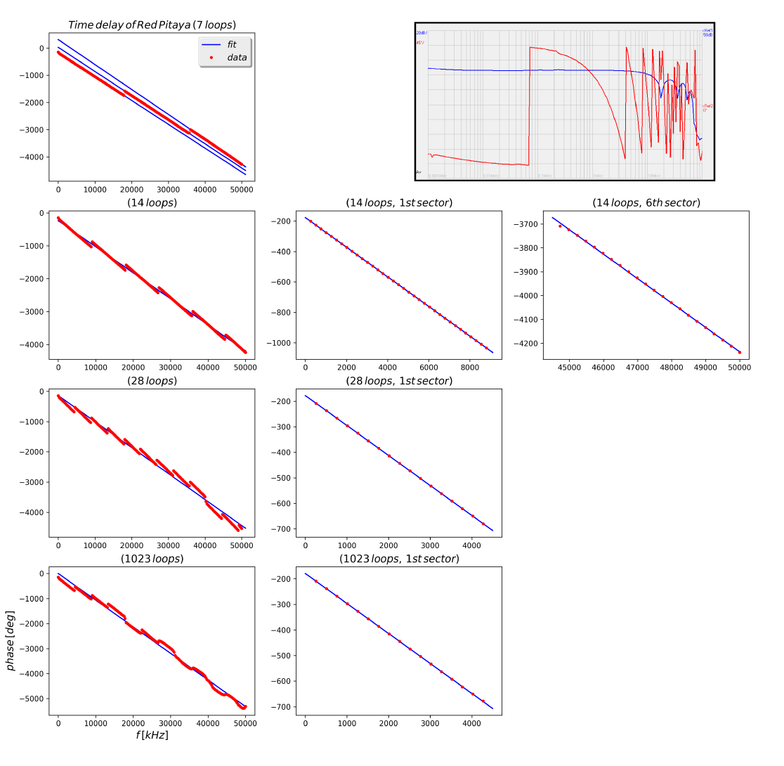
Figure 4: Time Delay. As we can see, the number of loops determines the number of jumps the phase does: I estimated that every time the phase changes by 100 deg, but also this value is affected by the number of loops. I called "sector" the straight line before the phase jumps.Above each chart the number of loops is indicated. The chart taken from the NA, which is the one in the upper right corner, displays the phase trend.
Another issue was the time delay introduced by the instrument. According to the data sheet, the sampling rate of the Red Pitaya is 20 clocks @ 125 MHz, which corresponds to a delay of the order of 20/125MHz = 0.16 micro seconds.
After eliminating connections that could increase the delay, the Network Analyser was connected to the Red Pitaya, which generated at transfer functions. I could change two parameters: the loops, which are defined as the decimation factor of IIR w.r.t. 125 MHz (at least they must be 3 - 5), and the gain, which I set to 0.27.
In Fig. 4 are shown the data and the best fit with delay 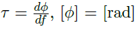 , given by:
The notation  loops sector has been used. As we can see, the time delay is not constant but depends on the number of loops, nevertheless it is consistent with what we expected.
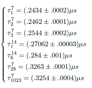
PI controller
Figure 5: PI controller. I had some problems with the chart in the upper left corner for two reason: around the "elbow" the points didn't fit well, while the plateau was not properly at (it was a little inclined with angular coefficient equal to 0.67 ms).
The next step was to create a more sophisticated typology of filters, the PI controllers. The transfer function of a PI is presented in the equation below.
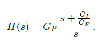
For the limits of PyRPL, I could just put the pole at a minimum of 10 Hz. In Fig. 5 there are some attempts I made to change their principal parameters that are the corner frequency, G_P and G_I ; in particular,
in order to change G_I, I had to insert another zero to Eq. 5: in this way I was able to easily decrease the slope of about 33% and increase it by approximately 50% with respect to the one I made first.
Homodyne Detection
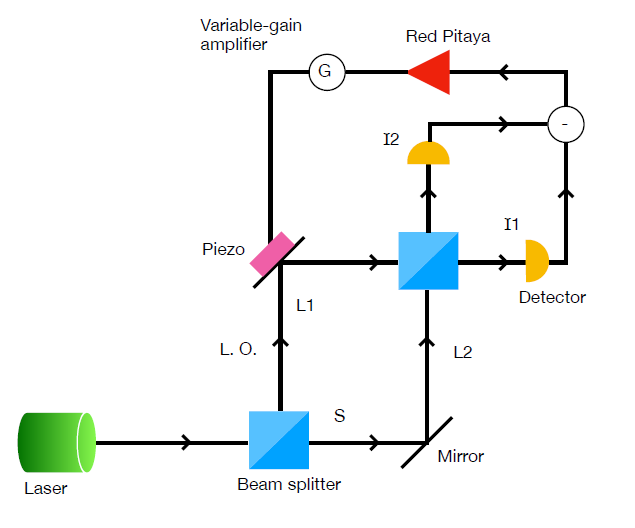
Figure 6: Optical set-up schematics.
The last part of the experiment was to apply knowledge of the board to a physical system, a Mach-Zehnder interferometer which is represented in Fig. 6. In order to measure the phase of an electric field we use interference, introducing another field called local oscillator, which represents the reference system (we will understand why shortly). The two fields are described by the equation below, when E_s is much larger than E_l.

The detectors then measure the intensity, according to this equation below.
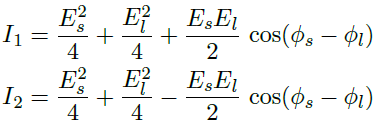
Where the minus sign in the second equation is due to the fact that the electric field undergoes a half-Pi phase shift when it crosses a medium with a higher index of refraction. Subtracting member to member the two equations we obtain something like,
As a consequence, we would like 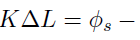
 , where
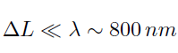
  is the arm length difference, to be zero: this occurs with very good approximation when:
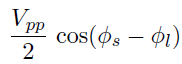
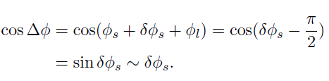
Only the thermal drift is greater, then a piezo is used to move one of the two mirrors: a piezo is an object that dilates and contracts in response to an electrical signal, moving the mirror by 1 micro meter if it applies 150 V. So before studying the phenomenon of interest, this contribution has to be eliminated. In this regard, a feedback loop is used via a PI controller, so the piezo tries to correct the error signal of the moving mirror to which it is applied with a speculative signal in some sense. Doing it around zero means measuring:
I added a gain amplifier between the Red Pitaya and the piezo, because the output voltage of the Red Pitaya was just 2 V_pp, so that the integrator saturated soon and the system was not stable.
I managed to lock the system within 1% of the error (qualitatively speaking, there were peaks of about 200 mV, while the resolution of the locking was 2 mV) for (1580  5) s, so for about 25 min. This part was made with the PID module, via GUI; actually I also tried via API or with the lockbox module, but I didn't succeed.
Physics.Benjamin
If you liked this post feel free to UPVOTE, FOLLOW, and RESTEEM.

References:-
[1] Red Pitaya
[2] L. Neuhaus. \PyRPL." (2016). URL:- https://github.com/lneuhaus/ pyrpl.
[3] L. Neuhaus. \Cooling a macroscopic mechanical oscillator close to its quantum ground state." Physics [physics]. Universite Pierre et Marie Curie - Paris VI (2016). English. NNT : 2016PA066555.
[4] Xilinx. \Zynq-7000 All Programmable SoC Overview." Technical report, Xilinx (2016).
[5] http://pyrpl.readthedocs.io/en/latest/#.
All have been made by myself, no copyright infringements have occurred.
Being A SteemStem Member
Congratulations! This post has been upvoted by SteemMakers. We are a community based project that aims to support makers and DIYers on the blockchain in every way possible. Find out more about us on our website: www.steemmakers.com.
If you like our work, please consider upvoting this comment to support the growth of our community. Thank you.
Congratulations @physics.benjamin! You have completed some achievement on Steemit and have been rewarded with new badge(s) :
Click on any badge to view your own Board of Honor on SteemitBoard.
To support your work, I also upvoted your post!
For more information about SteemitBoard, click here
If you no longer want to receive notifications, reply to this comment with the word
STOPPretty nice board for a fair price.
A more generic one that may be interesting based on the same SoC: https://steemit.com/technology/@boucaron/super-affordable-arm-9-fpga-developing-hardware-made-easier
For laser detection, do you have some links for cheap power measurement sensors for UV Laser (around 405nm) ?